PythonとKerasによるディープラーニングを読み進める その１の続きです。
今日はいよいよmnist以外のサンプルを実行します。

IMDbデータセット

• 50,000件の映画レビューのデータセット
• 「肯定的」または「否定的」というラベルが用意されている。
• 訓練用データ: 25,000件
• テストデータ: 25,000件

IMDbデータセットのインポート

from keras.datasets import imdb
(train_data, train_label), (test_data, test_label) = imdb.load_data(num_words=10000)

num_wordsという引数は、出現頻度の高いnum_words個のデータ以外捨てるということを表している。

print(train_data[0])
print(train_label[0])
---
[1, 14, 22, 16, 43, 530, 973, 1622, 1385, 65, 458, 4468, 66, 3941, 4, 173, 36, 256, 5, 25, 100, 43, 838, 112, 50, 670, 2, 9, 35, 480, 284, 5, 150, 4, 172, 112, 167, 2, 336, 385, 39, 4, 172, 4536, 1111, 17, 546, 38, 13, 447, 4, 192, 50, 16, 6, 147, 2025, 19, 14, 22, 4, 1920, 4613, 469, 4, 22, 71, 87, 12, 16, 43, 530, 38, 76, 15, 13, 1247, 4, 22, 17, 515, 17, 12, 16, 626, 18, 2, 5, 62, 386, 12, 8, 316, 8, 106, 5, 4, 2223, 5244, 16, 480, 66, 3785, 33, 4, 130, 12, 16, 38, 619, 5, 25, 124, 51, 36, 135, 48, 25, 1415, 33, 6, 22, 12, 215, 28, 77, 52, 5, 14, 407, 16, 82, 2, 8, 4, 107, 117, 5952, 15, 256, 4, 2, 7, 3766, 5, 723, 36, 71, 43, 530, 476, 26, 400, 317, 46, 7, 4, 2, 1029, 13, 104, 88, 4, 381, 15, 297, 98, 32, 2071, 56, 26, 141, 6, 194, 7486, 18, 4, 226, 22, 21, 134, 476, 26, 480, 5, 144, 30, 5535, 18, 51, 36, 28, 224, 92, 25, 104, 4, 226, 65, 16, 38, 1334, 88, 12, 16, 283, 5, 16, 4472, 113, 103, 32, 15, 16, 5345, 19, 178, 32]
1

train_data[0]の中身を見ると、どうやらあらかじめ単語をインデックス(int)に置き換えて格納しているようだ。
また、10000個の単語を抽出しているため、単語のインデックスが10000を超えることはない。

print(max([max(sequence) for sequence in train_data]))
---
9999

IMDbデータセットのdecode

整数の配列として表現されているものを映画レビューに復元する。

word_index = imdb.get_word_index()
reverse_word_index = dict([(value, key) for (key, value) in word_index.items()])
# `i-3`となっているのは0, 1, 2がそれぞれ「パディング」「シーケンス開始」「不明」のインデックスとして予約されているため
decord_review = ' '.join([reverse_word_index.get(i - 3, '?') for i in train_data[0]])

print(decord_review)
---
? this film was just brilliant casting location scenery story direction everyone's really suited the part they played and you could just imagine being there robert ? is an amazing actor and now the same being director ? father came from the same scottish island as myself so i loved the fact there was a real connection with this film the witty remarks throughout the film were great it was just brilliant so much that i bought the film as soon as it was released for ? and would recommend it to everyone to watch and the fly fishing was amazing really cried at the end it was so sad and you know what they say if you cry at a film it must have been good and this definitely was also ? to the two little boy's that played the ? of norman and paul they were just brilliant children are often left out of the ? list i think because the stars that play them all grown up are such a big profile for the whole film but these children are amazing and should be praised for what they have done don't you think the whole story was so lovely because it was true and was someone's life after all that was shared with us all

1. imdb.get_word_index()で単語をkey、インデックスをvalueとしたdictを取得できる
2. reverse_word_indexでインデックスのkeyに、単語をvalueに入れ替えたdictを作成
3. reverse_word_indexをもとにインデックスの配列を単語に置き換え、文字列結合を行う

one-hot表現に変換

import numpy as np

def vectorize_sequences(sequences, dimension=1000):
    results = np.zeros((len(sequences), dimension))
    for i, sequence in enumerate(sequences):
        results[i, sequence] = 1
    return results

x_train = vectorize_sequences(train_data)
x_test = vectorize_sequences(test_data)

enumerateを使うと、for文をindex付で回すことができる。
また、results[i, sequence]の部分だが、numpyの配列は以下のようにインデックスを配列で指定して取得ができる。
知らなんだ。

a = np.array([[0, 1, 2], [3, 4, 5], [6, 7, 8]])
print(a[1, [1, 2]])
---
[4 5]

one-hot表現に変換することで、単語の並び順の情報を消えるのだが、良いのだろうか。
並び順が肯定的/否定的の判断に、意味があるかどうかは探索的データ分析を行った上での判断する必要がありそう。
また、ラベルもベクトル化しておく。

y_train = np.asarray(train_labels).astype('float32')
y_test = np.asarray(test_labels).astype('float32')

ニューラルネットワークを構築

from keras import models
from keras import layers

model = models.Sequential()
model.add(layers.Dense(16, activation='relu', input_shape=(10000, )))
model.add(layers.Dense(16, activation='relu'))
model.add(layers.Dense(1, activation='sigmoid'))

model.compile(optimizer='rmsprop', loss='binary_crossentropy', metrics=['accuracy'])

ネットワークの定義

今回のような単純な入力には、単純な全結合層(Dense)のスタックとReLU活性化関数で構成されたネットワークが良い。

Dense(16, activation='relu')

ここで行われる計算は以下の通りであり、Wとinputの内積により、入力データは16次元の表現空間に射影される。
つまりWの形は(16, 10000)となっている。

output = relu(dot(W, input) + b)

Dense層を使用する場合、アーキテクチャ上、2つの重要な意思決定が必要である。
この意思決定のガイドラインは4章で説明されるそう。

• 使用する層の数をいくつにするか
• 各層の隠れユニットの数をいくつにするか

今回の例では、以下の通りのネットワークになっている。

• それぞれ16個の隠れユニットを持つ2つの中間層
• 現在のレビューの感情に関する予測値(スカラー)を出力する3つめの層

ネットワーク定義のコンパイル

model.compile関数で損失関数とオプティマイザの指定を行う。

二値分類問題のセオリー

• 損失関数: binary_crossentropy(二値の交差エントロピー)
• オプティマイザ: rmsprop

交差エントロピーとは以下の式で表される損失関数。

確率を出力するときは交差エントロピーが最適とのこと。

モデルの訓練

データの準備

訓練データを訓練用と検証用に分割する。
25,000個のサンプルのうち、15,000を訓練用、10,000を検証用とする。

x_val = x_train[:10000]  # 訓練用
partical_x_train = x_train[10000:]  # 検証用

y_val = y_train[:10000]  # 訓練用
partical_y_train = y_train[10000:]  # 検証用

512サンプルのミニバッチで20エポックの訓練を行う処理は以下の通り。

history = model.fit(partical_x_train, partical_y_train, epochs=20, batch_size=512, validation_data=(x_val, y_val))

各エポックの最後に10,000個の検証データで損失率と正解率の計算を行う。
学習履歴、history.historyに格納されているので、matplotlibを使って可視化できる。

import matplotlib.pyplot as plt

history_dict = history.history
loss_values = history_dict['loss']
val_loss_values = history_dict['val_loss']

epochs = range(1, len(loss_values) + 1)

plt.plot(epochs, loss_values, 'bo', label='Training loss')
plt.plot(epochs, val_loss_values, 'b', label='Validation loss')
plt.title('Training and validation loss')
plt.xlabel('Epochs')
plt.ylabel('Loss')
plt.legend()
plt.show()

まずは損失関数の推移。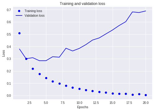

訓練用データに対する損失関数は20エポックを通して下がり続けているが、検証データに対しては4エポック目あたりで最小値になっている。
これは過学習(overfitting)と呼ばれる問題で、訓練データに以外のデータに対する予測率が落ちてしまっている状態である。
この場合、訓練のエポック数を減らして(今回の場合は4にして)再実行することでoverfittingを防ぐことができる。
ちなみに、正答率もグラフ化できる。

acc = history_dict['acc']
val_acc = history_dict['val_acc']

plt.plot(epochs, acc, 'bo', label='Training acc')
plt.plot(epochs, val_acc, 'b', label='Validation acc')
plt.title('Training and Validation accuracy')
plt.xlabel('Epochs')
plt.ylabel('Accuracy')
plt.legend()
plt.show()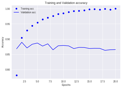

今日はここまで！